Vehicle Detection and Tracking

Outline

• Perform a Histogram of Oriented Gradients (HOG) feature extraction on a labeled training set of images and train a classifier Linear SVM classifier
• Apply a color transform and append binned color features, as well as histograms of color, to your HOG feature vector.
• Normalize your features and randomize a selection for training and testing.
• Implement a sliding-window technique and use the trained classifier to search for vehicles in images.
• Run the pipeline on a video stream and create a heat map of recurring detections frame by frame to reject outliers and follow detected vehicles.
• Estimate a bounding box for vehicles detected.

Histogram of Oriented Gradients (HOG)

1. Extract HOG features from the training images

In detect.ipynb, extract_features function calls get_hog_features function to extract HoG features from training images.

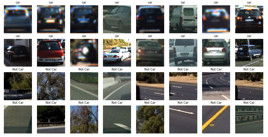
I started by reading in all the vehicle and non-vehicle images. Below is shown few example images from the vehicle and non-vehicle classes:

Next, I experimented with different color spaces as well as different sklearn.hog parameters like orientation, pix_per_cell, cell_per_block and so on. Eventually I narrowed down the parameter values so as to achieve best accuracy on test data.

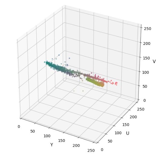
I used YUV color space which looks like this:

Here is an example using the YUV color space and HOG parameters of orientations=11, pixels_per_cell=(16, 16) and cells_per_block=(2, 2):

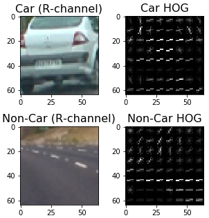
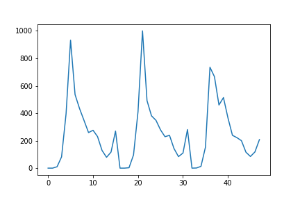
Figure below shows Histogram Feature of bbox-example-image

2. Choice of HOG parameters

I experimented with different values of each parameter, each time evaluating the accuracy on the test set and correctness on the given test video. Later tuning for some parameters was required when working with the actual project video.

Train a classifier

From the Raw image data, I extracted the 3-channel spatial color, histogram and HoG features. After spliting the entire feature data into test and train data, I created a Linear SVM object. This SVM was trained using 80% of the total data to result in 98.56 % accuracy on Test set. All immediate predictions were on point. This part is marked as Training a SVM in the detect code.

Sliding Window Search

1. Sliding window search

Instead of using sliding window of different sizes, I used different scaling of the feature image. Thus with a fixed window size of 64 pixels, I iterated over every 2 cell steps. All 3 type of Features were extracted along each window and fed to the predict function of my SVC after realigning. If prediction was 1 (i.e. Car), I recorded the window. I experimented with different scales and decided to use gradually increasing scale as we move towards the bottom of the image. However, the overlap was fixed to 2 cell steps.

The image area covered by different scales is shown below.

2. Testing and performance optimizations

Sliding the window over the entire image is time_consuming and redundant. Since car can only appear at the bottom half of any image, I constarined my window search to only bottom part. Moreover, the cars appear to be smaller at the upper part as compared to the bottom-most part. Therefore I used different scaling throughout the bottom half of the test image. This reduced the number of window iterations dramatically and improved performance of classifier.

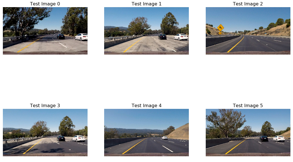
Here are some example images:

Video Implementation

TODO

Filter and Combine

The function find_cars return a list of all bounding boxes where a car was found. However, this list contains many false positives. To tackle this, I first combined all overlapping boxes by adding on top of each other to generate a heatmap of detections. This is implemented in function add_heat. Stronger the value of heat at point, more are the chances that multiple windows overlapped to give a positive detection at this point. Thus I thresholded this heatmap in apply_threshold function to only keep strong detections. label function returns all the bounding boxes from the thresholded heatmap. These boxes are then plotted using draw_labeled_bboxes function.

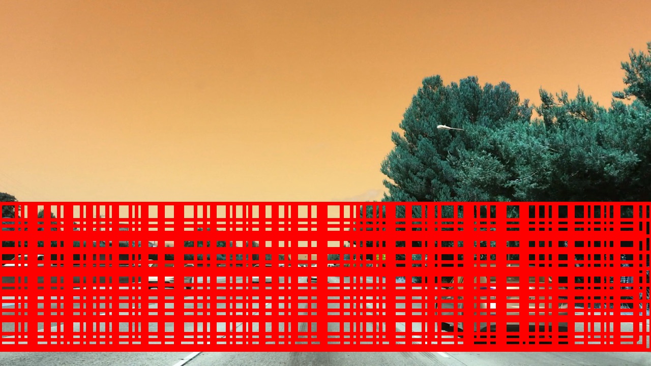
Following image was taken from a processed Video. Noisy Heatmap is shown in the top-left corner and Filtered Heatmap is shown in the top-right corner:

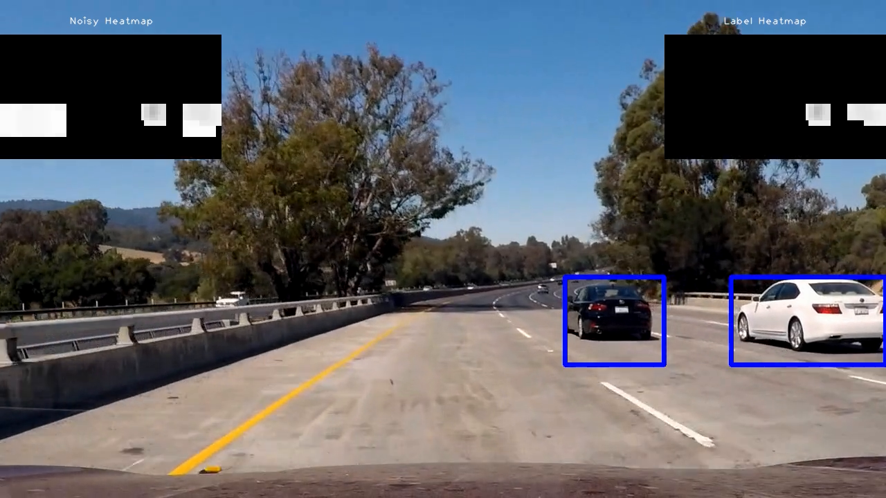
Here’s an example result showing the heatmap from a series of frames of video, the result of scipy.ndimage.measurements.label() and the bounding boxes then overlaid on the last frame of video:

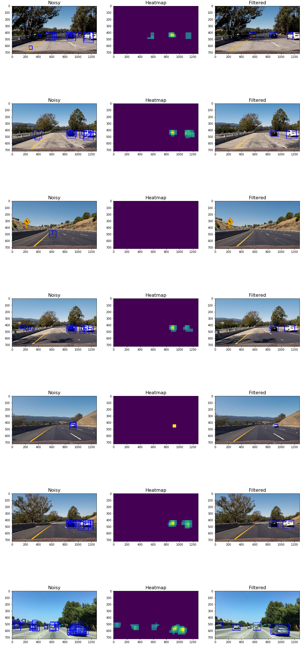
Output images

Here are six frames and their corresponding Noisy detections, heatmaps and label or filtered output:

Discussion

The only thing that took most of my time was tuning the HoG parameters for optimum detection. One case where my pipeline is likely to fail is when the plane of the road is different then the project video. As I have truncated the top half part of the frame, any vehicle in that part won’t be detected. Apart from this, lightning conditions might affect the detection.