Lane-line Segmentation
Outline
- Compute the camera calibration matrix and distortion coefficients given a set of chessboard images.
- Apply a distortion correction to raw images.
- Use color transforms, gradients, etc., to create a thresholded binary image.
- Apply a perspective transform to rectify binary image (“birds-eye view”).
- Detect lane pixels and fit to find the lane boundary.
- Determine the curvature of the lane and vehicle position with respect to center.
- Warp the detected lane boundaries back onto the original image.
- Output visual display of the lane boundaries and numerical estimation of lane curvature and vehicle position.
TODO video
Camera Calibration
The function calibrate() in the lane_finder.py is used to find camera calibration matrix and coefficients. To acheive this we first define object points which are the true position of corners of the chessboard to be used for calibration. We then find the image points (or corners) from the uncalibrated image using the function findChessboardCorners().
Once we have the object and image points, we call the function calibrateCamera() to obtain the calibration matrix and coefficients. These calibration parameters are later used in undistort() function to remove distortion incurred through camera.
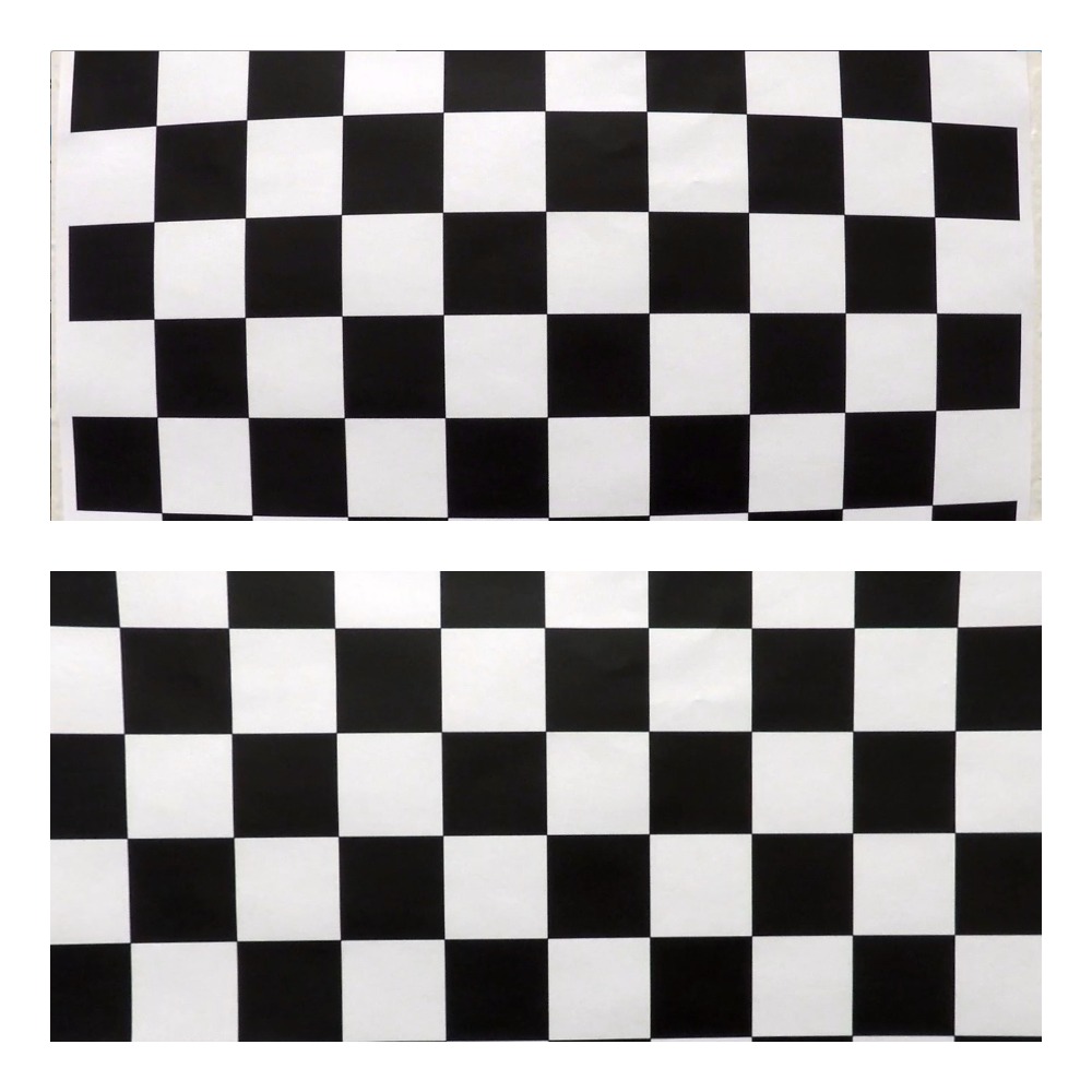
An example distortion-correction on one of the chessboard image is shown below,
Pipeline (single image)
1. Distortion-corrected image
Henceforth we will be using the following iamge (distortion-corrected) to demonstrate all transformations: 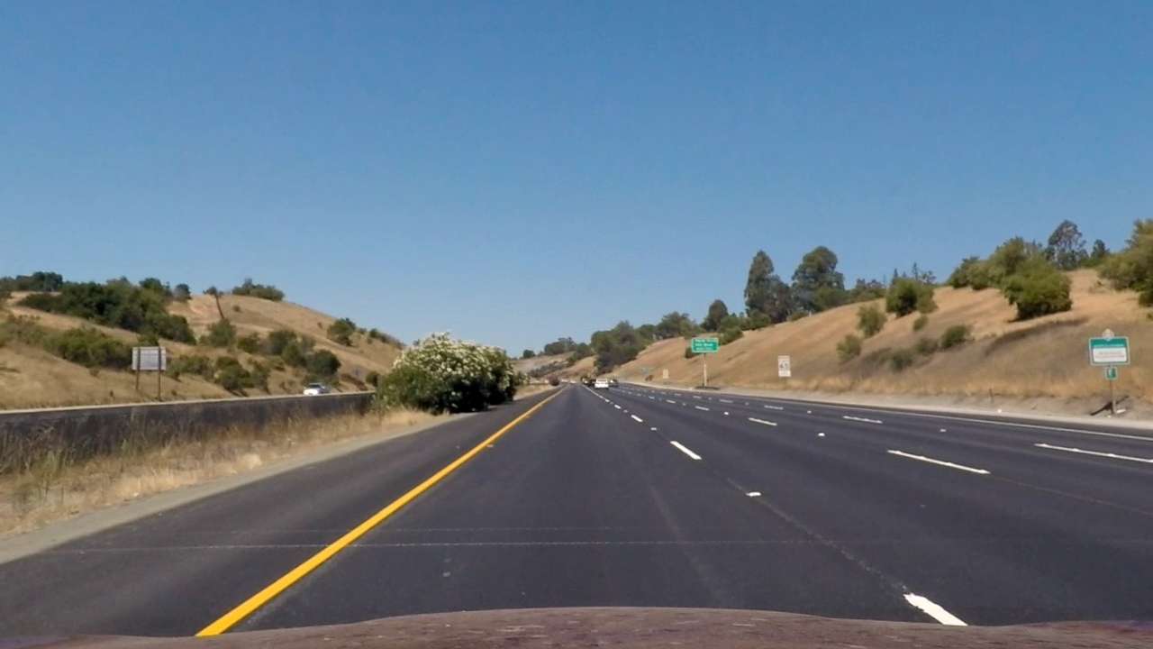
2. Color transforms, gradients or other methods to create a thresholded binary image
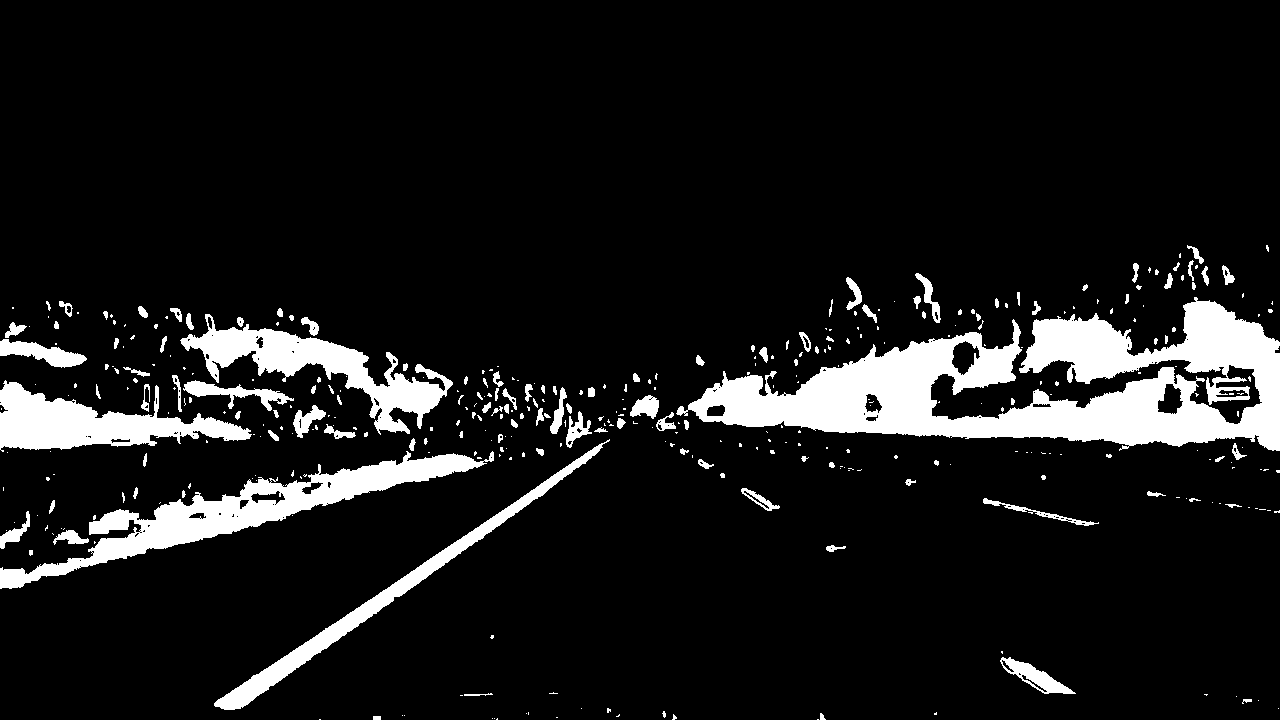
In the lane_finder.py program, the get_warped() function is used for obtaining a combined binary thresholded image. For the project video, I have used the following color spaces to threshold the original frame. 1. Sobel gradient on L channel of Lab color space 2. Simple thresholding of HLS color space 3. Simple thresholding of B-channel of Lab color space These three thresholded images then were combined to obtain a final binary image which clearly highlights lane-lines on both sides. The following image shows the final thresholded image obtained:
3. Perspective transform
After obtaining the binary image in the get_warped() function, I selected best source points that can be used for perspective transform. These source points then have to be transformed to to predefined destination points. The function getPerspectiveTransform() takes source and destination points as input and returns a transform matrix which can then be used by warpPerspective() function to give a perspective transformed image. I have used the following points as src and dest.
src = np.float32(
    [[210, img.shape[0] - 1],
    [595,450],
    [690,450],
    [1110, img.shape[1] - 1]])
dest = np.float32(
    [[200, img.shape[0] - 1],
    [200,0],
    [1000,0],
    [1000, img.shape[1] - 1]])
This resulted in the following source and destination points:
| Source | Destination |
|---|---|
| 210, 759 | 200, 759 |
| 595, 450 | 200, 0 |
| 690, 450 | 1000, 0 |
| 1110, 1279 | 1000, 1279 |
The source points when drawn on the original image, the src lines are almost parallel to the lane lines as can be seen here, 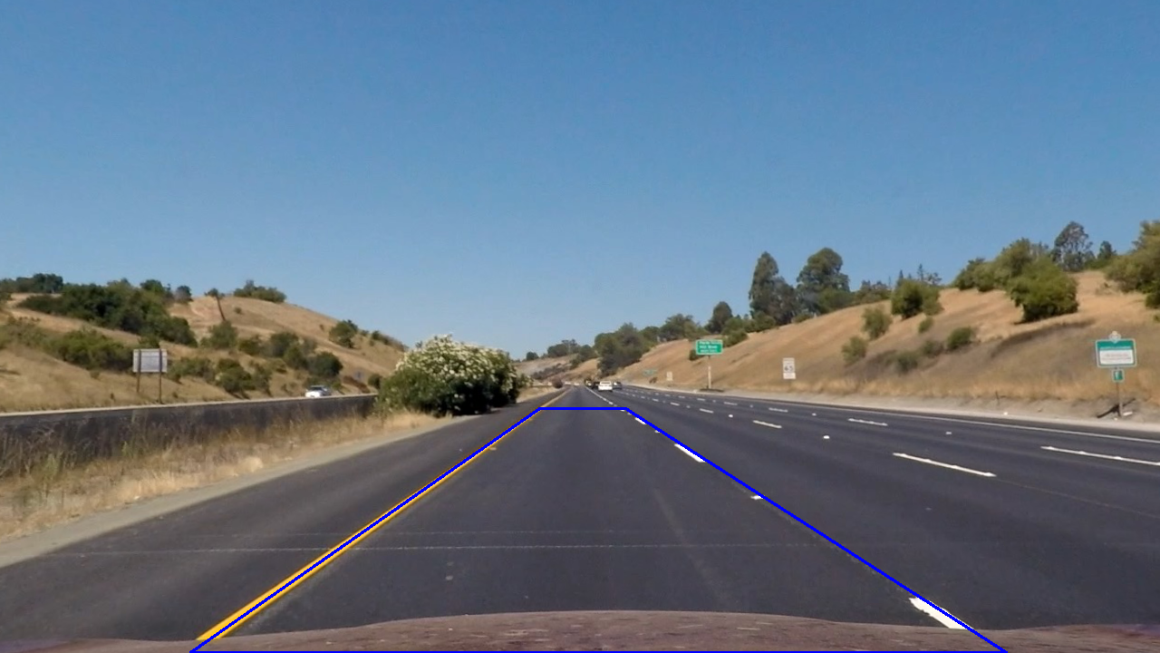
After applying perspective transform to our selected image, the src lines become parallel to each other as they are supposed to be when viewed from top. 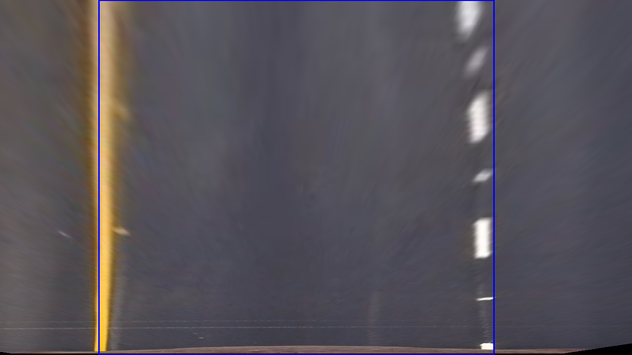
4. Identify lane-line pixels and fit their positions with a polynomial
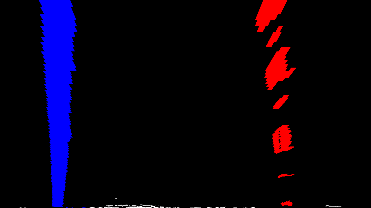
This is done at to places in my code, one is in the slide_window() function and the other is in the looper() function. As we start in slide_window() by finding the peak point in histogram of a sub-image, we later all the points located near this peak. In this way all the points located on the lane lines are obtained which are then passed to polyfit() to obatin coefficients of polynomial. Below I have shown the detected pixels on both lane-lines in different color:
5. Calculate the radius of curvature of the lane and the position of the vehicle with respect to center
In my code, this is done in the looper() function. I first converted my lane points to meter metric using the conversion given in the course module. This was followed by applying a second order radius of curvature formula which is nicely explained here: https://www.intmath.com/applications-differentiation/8-radius-curvature.php
6. Result plotted back down onto the road such that the lane area is identified
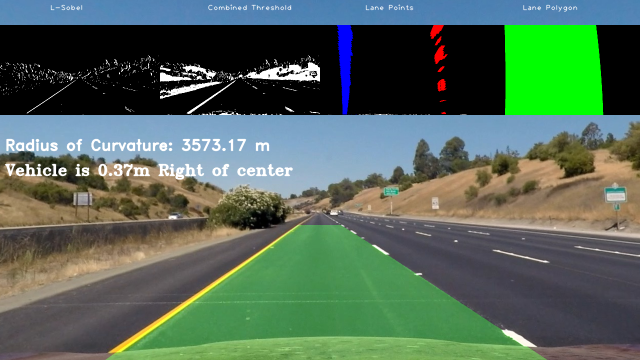
This has been implemented in the looper() function. Here, we use the perspective transform matrix to get reverse the transform and obtain the camera view image with the lane polygon plotted in green.
Pipeline (video)
TODO
Discussion
One problem is finding the suitable color spaces to obtain a binary output that contains almost all pixels of the lanes. This pipeline was picking a lot of points from non-lane pixels which was corrected using B-channel thresholding from Lab color space.
The pipeline is likely to fail when there are many color and shade changes between the two lanes. As the gradient will pick these points and include in the lane points thus resulting in undesirable detection. This could be solved by trying out different color space thresholing such that only lanes are present in the final bianry image. Further improvements can also include smoothing the detection using points history and also predicting the immediate curvature beforehand.